Who Learns Faster With Less Data? Adapters Beat Full Fine‑Tuning

Table of Links

Abstract and 1. Introduction

1. Related Work
2. Preliminaries
3. Experiments
4. Analysis
5. Conclusion, Limitations, and References

A. Reproducibility

3 Preliminaries

We now describe the experimental setup, providing details on the datasets as well as the PEFT and AL methods used in our study.

\

3.1 Datasets

We employ four single-text classification tasks commonly used for AL evaluation: (1) the subjectivity dataset (SUBJ; Pang and Lee, 2004), designed to assess the subjectivity of a given text; (2) the question type classification dataset (TREC; Li and Roth, 2002), designed for categorizing questions according to their types; (3) the Stanford Sentiment Treebank (SST; Socher et al., 2013), which focuses on sentiment analysis; (4) AG’s news classification dataset (AGN; Zhang et al., 2015), which classifies news articles into different categories. We provide the dataset statistics in the appendix for further reference (cf. Appendix Table 3)

\

3.2 PEFT methods

We consider four prototypical PEFT techniques:

\ Adapter incorporates trainable bottleneck layers after both the multi-head attention and feedforward block in each Transformer layer (Houlsby et al., 2019);

\ Prefix-tuning adds new parameters in the multihead attention blocks within each Transformer layer (Li and Liang, 2021);

\ LoRA (Low-rank adaptation) represents an additive method that incorporates trainable lowrank decomposition matrices into the layers of a pre-trained model (Hu et al., 2022);

\ UniPELT combines multiple PEFT approaches, namely LoRA, Prefix-tuning, and Adapter, in a single unified setup (Mao et al., 2022). Each constituent is a submodule, and UniPELT employs gating mechanisms to activate them effectively

\ All of the above PEFT methods fall under the category of lightweight fine-tuning. While prefixtuning does not technically qualify as an adapter, He et al. (2022) demonstrated that it shares formal similarities with adapters, with prefix-tuning performing weighted addition and an adapter employing unweighted addition. We refer to all four considered methods as adapters for terminological simplicity. We use BERT (Devlin et al., 2019) as the base PLM for every adapter. Additionally, we adhere to the hyperparameter settings for each adapter as recommended in the respective papers that introduced them (cf. Appendix A.2 for details).

\

3.3 AL methods

Our study considers five sampling strategies, including random selection (RND) as a passive learning baseline. The other four strategies are AL methods originating from different families, chosen for their robustness (ability to perform well across various tasks) and widespread usage in the field:

\ Maximum entropy (ENT; Lewis and Gale, 1994) comes from the family of uncertainty strategies. The method queries instances where the model is least certain based on the maximum entropy criterion of the prediction output;

\ Monte Carlo dropout (MC; Gal and Ghahramani, 2016) resembles ENT but utilizes the stochasticity of forward passes with dropout layers (Srivastava et al., 2014) to estimate the entropy for a given instance;

\ Monte Carlo dropout (MC; Gal and Ghahramani, 2016) resembles ENT but utilizes the stochasticity of forward passes with dropout layers (Srivastava et al., 2014) to estimate the entropy for a given instance;

\ Core-set (CS; Sener and Savarese, 2018) encourages instance diversity by using the learned representations of the acquisition model. This method aims to minimize the distance between an example in the unlabeled set and its closest counterpart in the labeled subset;

\ Discriminative active learning (DAL; Gissin and Shalev-Shwartz, 2019) frames AL as a binary classification of instances into those that are labeled and those that are not, with the objective of making the labeled and unlabeled sets indistinguishable.

\

3.4 Experimental setup

In AL runs, we select 50 new examples in each step of each AL experiment, using 100 examples for the warm start (randomly sampled labeled data to initiate the model). To probe different PEFT approaches with and without AL in low-resource settings, we establish a labeling budget limit of 1, 000 instances. To sidestep the need for a validation set in our experiments, which is typically unavailable in real-world AL scenarios, we adopt the Besov early stopping (Jukic and Šnajder ´ , 2023). This method utilizes the smoothness of Transformer layers to decide at which epoch to stop training.

\ In the case of TAPT, we pre-train the base model on a masked language modeling task using unlabeled training data. For adapters, we only update the injected parameters while keeping the remaining parameters of the base model frozen. This approach aligns with the primary function of adapters, which is to utilize a common base model across diverse tasks. For every setting, we perform five runs using different random seeds. We report the average F1 score at each sampling step (with and without AL for FFT and PEFT) to show the corresponding learning curve averaged over five runs. We provide details on training and hyperparameters in Appendix A.5.

\

3.5 Evaluation

To evaluate the overall performance of an AL method, we employ the area under the performance curve (AUC). In each individual AL step with a specific quantity of labeled examples, we measure the classification performance in terms of the F1 score. The overall AUC is calculated using the F1 scores obtained at each step. We advocate for using AUC alongside the AL curves, as AUC serves as a suitable approximation of AL feasibility through a summary numeric score, as recommended in recent AL literature (Schröder et al., 2022; Jukic and ´ Šnajder, 2023).

\

\ Intuitively, RIPL estimates the proportion of maximum possible improvement achievable by a given AL method compared to the passive learning baseline. A score of 1 indicates the maximum theoretical improvement, which would be tantamount to attaining an F1 score of 1 in the initial sampling step and sustaining that score throughout all steps. Conversely, a negative score indicates that the AL method performs worse than passive learning.

\

4 Experiments

In this section, we first examine the performance of PEFT methods in comparison to FFT with passive learning and then proceed to analyze the application of PEFT in AL settings.

\

4.1 PEFT vs. FFT

Previous research on the use of adapters in low-resource settings (Li and Liang, 2021; Mao et al., 2022; He et al., 2021) has demonstrated that adapters perform comparably to, and sometimes even better than FFT. However, these findings were based on comparing FFT to a single adapter variant on a full dataset or evaluating the performance at only a few discrete points.

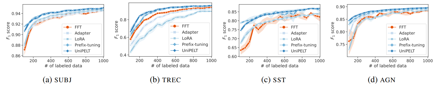
\ In the first part of our experiments, we build upon these findings by conducting a more nuanced analysis. We generate detailed learning curves that facilitate the comparison of multiple adapters with FFT under the passive learning setup. Our comparison, summarized by the AUC metric in Table 1, reveals that UniPELT and Prefix-tuning consistently outperform FFT with a significant difference across all datasets used in our study. Conversely, the performance of Adapter and LoRA is mostly comparable to FFT, although there are cases where they either outperform or underperform FFT. In cases in which Adapter and LoRA perform better than FFT with significant differences, the degree of improvement is smaller than what is observed with UniPELT and Prefix-tuning.

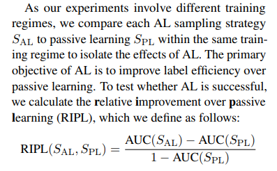
\ Next, we look into how the models’ performance changes as the training set increases. To that end, we show the corresponding learning curves for adapters and FFT in Figure 1. The performance disparities between adapters and FFT become more apparent under conditions of extreme data scarcity (100–300 labeled instances). Notably, the greatest differences in performance occur at the initial step (only 100 labels). This highlights the promise of adapter-based methods in low-resource settings, particularly for Prefix-tuning and UniPELT.

\

\

\

4.2 PEFT with AL

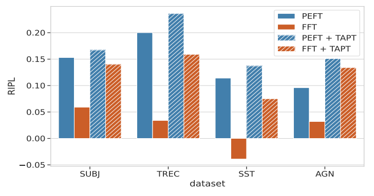
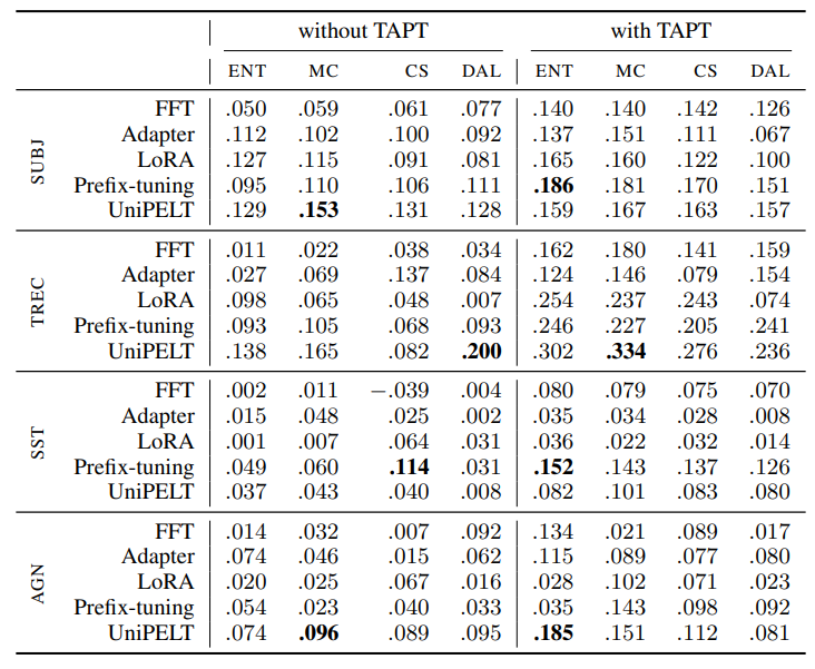
Motivated by our initial findings on using PEFT under the passive learning setup, where PEFT exhibited promising properties in low-resource settings, we further explore the behavior of adapters in AL scenarios. We evaluate individual PEFT methods in AL scenarios with and without using TAPT in terms of gains over random sampling (passive learning) using the RIPL metric described in Section 3.5. Table 2 shows the results for different combinations of AL methods and adapters, evaluated through the RIPL metric. We complement these results with absolute values in terms of AUC (cf. Appendix Table 5). For FFT without TAPT, DAL achieved the highest RIPL score on two datasets, while CS and MC topped the chart on one dataset each. When we incorporated TAPT, ENT yielded the best results on three out of four datasets, with CS leading on one. Looking at adapters, the most successful AL methods without TAPT vary, depending on the specific adapter and dataset in question. Interestingly, when TAPT is applied, the best results for all adapters are obtained either by ENT or MC. We speculate this could be attributed to solid compatibility between

\

\ entropy-based methods and TAPT when adapters are employed.

\ Furthermore, we observe that without TAPT, adapters achieve larger gains over FFT. However, when TAPT is applied, FFT becomes comparable to PEFT, although Prefix-tuning and UniPELT still yield the greatest improvements, depending on the dataset and AL method used. In Figure 2, we select the adapters that achieved the best improvement according to Table 2 without TAPT and show their RIPL value compared against FFT as well as their corresponding version when TAPT is applied. We conjecture that TAPT reduces the performance gap between adapters and FFT by inducing FFT to emulate PEFT in aspects such as training dynamics and representation space — a hypothesis we explore in more detail in Section 5.

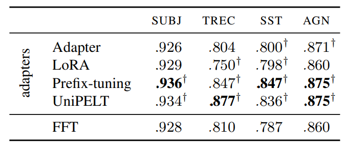
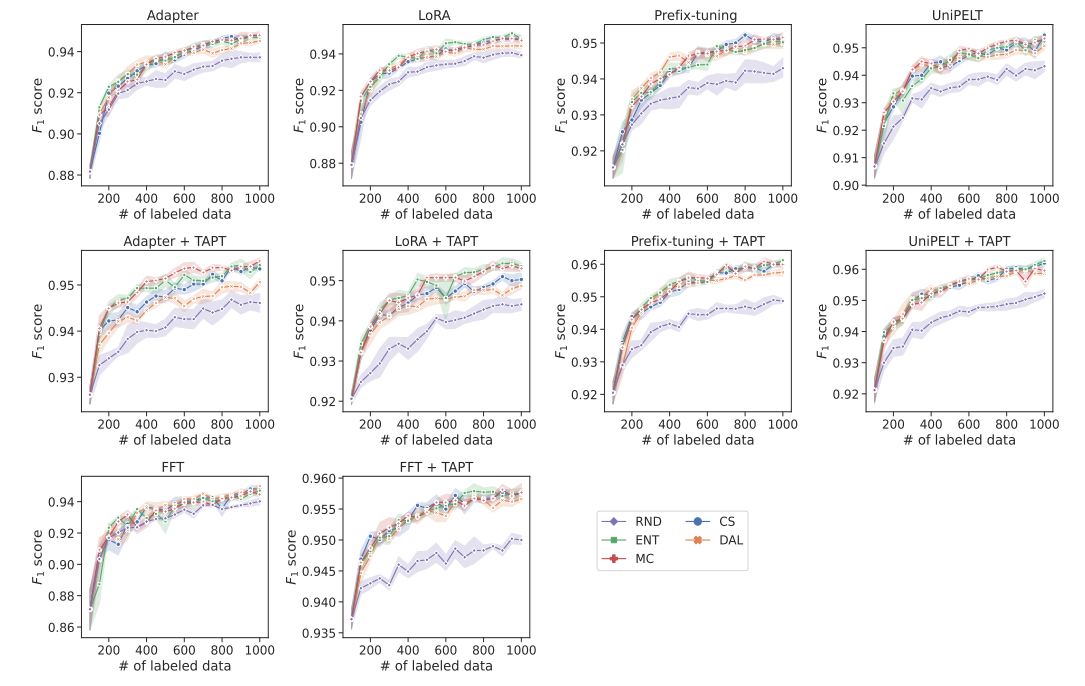
\ We further investigate the behavior of adapters with AL throughout the individual steps. Figure 3 shows the learning curves for corresponding adapter models with and without applying TAPT. Due to space constraints, we show the learning curves only for the SUBJ dataset, as similar trends occur for other datasets. Without TAPT, the performance of adapters is largely independent of the specific AL method used, where Prefix-tuning and UniPELT consistently outperform Adapter and LoRA across all AL steps. With TAPT, the differences between AL and random sampling are more pronounced starting from the early steps, typically already with 200 instances. In contrast, the gap becomes more apparent only with 500 or more instances when TAPT is not employed.

\

\

\

:::info Authors:

(1) Josip Jukic, Faculty of Electrical Engineering and Computing, University of Zagreb, Croatia (josip.jukic@fer.hr);

(2) Jan Šnajder, Faculty of Electrical Engineering and Computing, University of Zagreb, Croatia (jan.snajder@fer.hr).

:::

:::info This paper is available on arxiv under CC BY 4.0 DEED license.

:::

\